The ASAP Utilities menu in Excel (English)

Insert function from the ASAP Utilities library...
English (us) ⁄ Nederlands ⁄ Deutsch ⁄ Español ⁄ Français ⁄ Português do Brasil ⁄ Italiano ⁄ Русский ⁄ 中文(简体) ⁄ 日本語Formulas › 12. Insert function from the ASAP Utilities library...
With this utility you can insert a formula from the ASAP Utilities functions library into the active cell.The ASAP Utilities functions library includes the following functions:
=ASAPCELLCOLORINDEX(cell)
Returns the color index number of the cell.If you afterwards change the color in the cell, you have to press Control+Alt+F9 to have the formula recalculated.
Parameters:
# cell = The cell to get Excel's number for the fill color from.
=ASAPCOUNTBYCELLCOLOR(reference, color_index_nr)
Counts the number of cells in the given range that have a certain fill color.If you afterwards change the fill color in any of the referenced cells, you have to press Control+Alt+F9 to have the formulas recalculated.
Parameters:
# reference = The range of cells to search in.
# color_index_nr = The cell that has the fill color to count, or the color index number (1-56) from Excel.
=ASAPCOUNTBYFONTCOLOR(reference, color_index_nr)
Counts the number of cells in the given range that have a certain font color.If you afterwards change the font color in any of the referenced cells, you have to press Control+Alt+F9 to have the formulas recalculated.
Parameters:
# reference = The range of cells to search in.
# color_index_nr = The cell that has the font color to count, or the color index number (1-56) from Excel.
=ASAPCOUNTCHAR(within_text, find_text)
Counts the number of times a character occurs in a textThis way you can for example count the number of commas in a cell. This function is case sensitive.
Parameters:
# within_text = The text containing the character you want to count.
# find_text = The character to count the occurrences of. This has to be a single character.
=ASAPCOUNTSHADES(reference)
Counts the number of colored cells in your range.If you afterwards change the fill color in any of the referenced cells, you have to press Control+Alt+F9 to have the formulas recalculated.
Parameters:
# reference = The range of cells to count the number of cells that have a fill color.
=ASAPEXTRACTFILENAME(text, optional path_separator)
Returns the file name from a full path and filename. By default the formula uses a backslash (\) as separator, but optionally you can specify another separator.For example =ASAPEXTRACTFILENAME("D:\Projects\Archive\Client 1\Balance.xls") returns "Balance.xls".
Parameters:
# text = The value or cell address from which you want to extract only the file name
# path_separator = The path separator. Optional, if omitted a backslash (\) is used.
=ASAPEXTRACTFOLDERNAME(text, optional path_separator)
Returns the folder name from a combined filepath and filename. By default the formula uses a backslash (\) as separator, but optionally you can specify another separator.For example =ASAPEXTRACTFOLDERNAME("D:\Projects\Archive\Client 1\Balance.xls") returns "D:\Projects\Archive\Client 1".
Parameters:
# text = The value or cell address from which you want to extract only the folder name.
# path_separator = The path separator. Optional, if omitted a backslash (\) is used.
=ASAPEXTRACTNUMBERS(text_or_cell, optional keep_leading_zeros)
Returns the numbers from a text string.For example the formula =ASAPEXTRACTNUMBERS("8011 LB") returns 8011.
Parameters:
# text = The value or cell address from which you want to extract the numbers from.
# keep_leading_zeros = Optional. Preserve leading zeros. If omitted it is assumed to be TRUE.
=ASAPFILENAME()
Returns the name of your workbook. This is the name of the workbook without the filepath (folder).For example "Balance.xls".
=ASAPFILEPATH()
Returns the filepath (the folder) where your workbook is stored.For example: "D:\Projects\Archive\Client 1".
=ASAPFILEPROPERTIES(property_name_or_id)
Returns the value of one of the built-in document properties for the current workbook.You can refer to document properties either by index value or by their English name.
The following list shows the available built-in index values and document property names:
1 Title
2 Subject
3 Author
4 Keywords
5 Comments
6 Template
7 Last Author
8 Revision Number
9 Application Name
10 Last Print Date
11 Creation Date
12 Last Save Time
13 Total Editing Time *
14 Number of Pages *
15 Number of Words *
16 Number of Characters *
17 Security
18 Category
19 Format
20 Manager
21 Company
22 Number of Bytes *
23 Number of Lines *
24 Number of Paragraphs *
25 Number of Slides *
26 Number of Notes *
27 Number of Hidden Slides *
28 Number of Multimedia Clips *
29 Hyperlink Base
30 Number of Characters (with spaces) *
* Excel isn't required to define values for every built-in document property.
If Microsoft Excel doesn't define a value for one of the built-in document properties, reading the Value property for that document property results in an error.
You have to press Control+Alt+F9 to have the formula recalculated.
Example:
=ASAPFILEPROPERTIES("Last Print Date")
Parameters:
# property_name_or_id = The id or English name of the built-in document property
=ASAPFONTCOLORINDEX(cell)
Returns the color index number of the font of a cell.If you afterwards change the font color in the cell, you have to press Control+Alt+F9 to have the formula recalculated.
Parameters:
# cell = The cell to get Excel's number for the text color from.
=ASAPFULLFILENAME()
Returns the full filename of your workbook. This is the name of the workbook including the folder (filepath) where it is saved.For example "D:\Projects\Archive\Client 1\Balance.xls".
=ASAPGETCOMMENT(cell)
Returns the text from the comment a cell.If you afterwards change the comment in the cell, you have to press Control+Alt+F9 to have the formula recalculated.
Parameters:
# cell = The cell to get the text from the comment from.
=ASAPGETDOMAIN(text, optional show_protocol = False)
Returns the (sub)domain from a given hyperlink (website address/url).
For example if cell A1 contains the value "https://www.asap-utilities.com/download-asap-utilities.php" then these are the formula results:
=ASAPGETDOMAIN(A1) returns "www.asap-utilities.com"
=ASAPGETDOMAIN(A1;TRUE) returns "https://www.asap-utilities.com"
Parameters:
# text = The value or cell address from which you want to extract the domain.
# show_protocol = Optional, logical value, if omitted the default is FALSE. If TRUE this function will also return the protocol of the link, which is the part before the domain such as http://, ftp:// etc..
=ASAPGETFONTNAME(cell)
Returns the name of the font in a cell.If you afterwards change the font in the cell, you have to press Control+Alt+F9 to have the formula recalculated.
This function does not recognize formatting if it is applied via conditional formatting.
Parameters:
# cell = The cell to get the font from.
=ASAPGETFONTSIZE(cell)
Returns the font size of a cell.If you afterwards change the font size in the cell, you have to press Control+Alt+F9 to have the formula recalculated.
This function does not recognize formatting if it is applied via conditional formatting.
Parameters:
# cell = The cell to get the font size from.
=ASAPGETFORMULA(cell)
Returns the formula of a cell.Parameters:
# cell = The cell to get the formula from.
=ASAPGETFORMULAINT(cell)
Returns the formula of a cell in the "international" notation.The English names for the formulas will be used, the list separator is a comma and the decimal separator is a point.
The largest resources on the Internet on Excel are in English. On these websites the "international" formulas and style are used. If you use a local version of Excel you can now easily create an "international" example of the formula you used.
Parameters:
# cell = The cell to get the formula from.
=ASAPGETHYPERLINK(cell, optional text_no_link)
Returns the hyperlink from a cell. The hyperlink can be one of the following types:- existing file or web page
- place in your document
- e-mail address
If you afterwards change the hyperlink in the cell, you have to press Control+Alt+F9 to have the formula recalculated.
Parameters:
# cell = The cell to read the hyperlink from.
# text_no_link = Optional, this text will be displayed if the cell doesn't have a hyperlinks. If omitted, the formula will give an empty result for cells without hyperlinks.
=ASAPGETINDENTLEVEL(cell)
Returns the indent level for the cell.If you afterwards change the indent level in the cell, you have to press Control+Alt+F9 to have the formula recalculated.
Parameters:
# cell = The cell to get the indent level from.
=ASAPGETNUMBERFORMAT(cell)
Returns the number format of a cell.If you afterwards change the number format in the cell, you have to press Control+Alt+F9 to have the formula recalculated.
Parameters:
# cell = The cell to get the number format from.
=ASAPISBOLD(reference)
Returns TRUE if the cell is bold or FALSE if it isn't.If you afterwards change the bold setting in the cell, you have to press Control+Alt+F9 to have the formula recalculated.
=ASAPISFORMULA(cell)
Returns TRUE if the cell has a formula or FALSE if it doesn't.=ASAPLOADIMAGE(image_fullname, optional width_in_pixels, optional height_in_pixels)
Inserts the specified image as an object and puts it at the left-top of your cell.To update the image, you can replace the formula with a new image name.
To remove the image you have to remove both the formula and the image. (The image isn't removed if only the formula is removed.)
You have to press Control+Alt+F9 to have the formula recalculated.
Example:
=ASAPLOADIMAGE("D:\products\images\art782.gif")
Parameters:
# image_fullname = The full path and file name of an image of the type that Excel supports
# width_in_pixels = Optional. You can specify the width pixels. If omitted, the width will be proportionally based on the image's height
# height_in_pixels = Optional. You can specify the height in pixels. If omitted, the height will be the height of the cell the formula is in.
=ASAPMERGECELLS(reference, optional delimiter = "", optional skip_empty_cells = True)
Joins several text strings into one text string.An easy alternative for the Excel =CONCATENATE() function. The benefit of this ASAP Utilities function:
- You can specify a range to join, for example "A1:G1".
- The numberformat of the values will be used. For example if a cell has the value "12.23072" and the number format is to display only one decimal then this function uses the value "12.2".
- You only have to specify a delimiter once.
- By default empty cells will be ignored.
Parameters:
# reference = A contiguous range of cells to join the values from. When reading the cell values, their number format will be used.
# delimiter = Optional, a character to insert between the cell values. If omitted no delimiter is used.
# skip_empty_cells = Optional, is a logical value: to skip empty cells = TRUE or omitted; to include empty cells in the result = FALSE.
=ASAPRANDOMPASSWORD(optional length = 8, optional use_symbols = True)
Returns a random string that can be used as a password.This function will return a strong password which contains:
- both uppercase and lowercase letters
- numbers
- special characters, such as ~!@#$%^*()[]\/<>:-=+_
Parameters:
# length = Optional, the length of the password. If omitted the length will be 8 characters. If the length given is less than 8, still a password of 8 characters will be returned.
# use_symbols = Optional, is a logical value: to use special characters in the password = TRUE or omitted; to create a password without special characters = FALSE.
=ASAPREGEXMATCH(read_value, regular_expression, optional ignorecase)
Returns TRUE if the value matches the regular expression and FALSE if it does not.Parameters:
# read_value = The text to be tested against the regular expression.
# regular_expression = The regular expression to test the text against.
# ignorecase = Optional. Specifies case-insensitive matching. If omitted it is assumed to be FALSE.
=ASAPREGEXEXTRACT(read_value, regular_expression, optional ignorecase)
Returns the text that matches the regular expression.Parameters:
# read_value = The text to be tested against the regular expression.
# regular_expression = The regular expression to test the text against.
# ignorecase = Optional. Specifies case-insensitive matching. If omitted it is assumed to be FALSE.
=ASAPREGEXREPLACE(read_value, regular_expression, replacement_value, optional replace_all, optional ignorecase)
Returns a modified version of the text string based on a regular expression.Parameters:
# read_value = The text to be tested against the regular expression.
# regular_expression = The regular expression to test the text against.
# replacement_value = The text to replace the matched groups with.
# replace_all = Optional. Specifies to replace all matches. If omitted it is assumed to be TRUE.
# ignorecase = Optional. Specifies case-insensitive matching. If omitted it is assumed to be FALSE.
=ASAPSHEETNAME(optional reference)
Returns the name of the worksheet this formula is used on.Parameters:
# reference = Optional, a cell on the sheet that you want to get the name from. If omitted the name of the current sheet is returned.
=ASAPSPELLNUMBER(ByVal number, optional strLanguage = "EN", optional blnCurrency = False, optional strSingular, optional strPlural, optional strComma, optional strCentSingular, optional strCentPlural)
Returns a spelled-out number or amount.A few examples if cell A1 contains the value 142.23
=ASAPSPELLNUMBER(A1,"EN", TRUE, "Dollar", "Dollars", , "Cent", "Cents") returns One Hundred Forty-Two Dollars and Twenty-Three Cents
=ASAPSPELLNUMBER(A1,"EN", FALSE,,,"Comma") returns One Hundred Forty-Two Comma Twenty-Three Hundredths
=ASAPSPELLNUMBER(A1,"NL") returns honderdtweeënveertig en drieëntwintig honderdsten
=ASAPSPELLNUMBER(A1,"FR", TRUE, "euro", "euros", , "cent", "cents") returns cent quarante-deux euros et vingt-trois cents
=ASAPSPELLNUMBER(A1,"DE", TRUE, "Euro", "Euros", , "Cent", "Cent") returns einhundertzweiundvierzig Euros und dreiundzwanzig Cent
If a number contains more than two decimals this function will spell out the number as if it was rounded to two decimals.
A practical example where this function can be useful is to write out amounts on cheques.
Parameters:
# number = The number or cell with a number you want to spell.
# language = Optional, text string representing in which language the number is spelled out: English = EN or omitted, Dutch = NL, German = DE, French = FR.
# currency = Optional, logical value: to spell the number as a currency = TRUE; to spell the number just as a number = FALSE or omitted. For example spell the number 2 as "two dollars and no cents" or just "two".
# cur_singular = An optional text string for the currency spelled singular. For example "dollar".
# cur_plural = An optional text string for the currency spelled plural. For example "dollars".
# comma = An optional text string for the decimal separator used. For example the comma sign (",") or point (".") or the word "comma" or "and". If omitted then it will be automatically filled depending on the given language: English = "and", Dutch = "en", German = "und" and French = "et".
# cur_cent_singular = An optional text string for the word used with currency for the amount behind the comma, singular. For example "cent".
# cur_cent_plural = An optional text string for the word used with currency for the amount behind the comma, plural. For example "cents".
=ASAPSTRIPNUMBERS(text)
Removes all numbers from a text string and removes all spaces at the beginning and end of the result.For example the formula =ASAPSTRIPNUMBERS("8011 LB") returns "LB".
Parameters:
# text = The value or cell address from which you want to strip the numbers.
=ASAPSUMBYCELLCOLOR(reference, color_index_nr)
Adds the cells that have a certain fill color.If you afterwards change the color in any of the referenced cells, you have to press Control+Alt+F9 to have the formulas recalculated.
Parameters:
# reference = The range of cells to search in.
# color_index_nr = The cell that has the fill color to sum, or the color index number (1-56) from Excel.
=ASAPSUMBYFONTCOLOR(reference, color_index_nr)
Adds the cells that have a certain font color.If you afterwards change the font color in any of the referenced cells, you have to press Control+Alt+F9 to have the formulas recalculated.
Parameters:
# reference = The range of cells to search in.
# color_index_nr = The cell that has the font color to sum, or the color index number (1-56) from Excel.
Screenshots
Example screenshot: 1
Example screenshot: 2 Calculate the sum of cells that have a specific color

Example screenshot: 3 Retrieve the comments


Practical tricks on how this can help you
Practical 'real world' examples on our blog that show you how this tool can help you in Excel. Enjoy!Starting this tool
- Click ASAP Utilities › Formulas › 12. Insert function from the ASAP Utilities library...
- Specify a Keyboard Shortcut: ASAP Utilities › Favorites & Shortcut keys › Edit your favorite tools and shortcut keys...
Download an example workbook that shows how to use these extra functions.
We have created a workbook (in English) that shows practical examples of how to use all these extra worksheet functions: Example-workbook-ASAP-Utilities-8-0-formulas.xlsb (0.3 MB)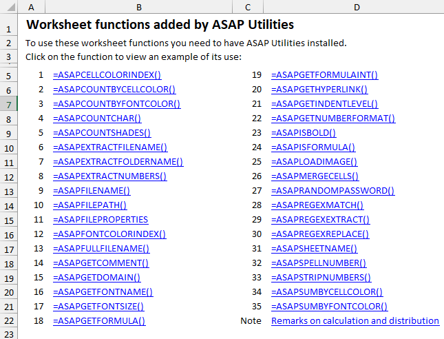
Important information on when Excel makes calculations and recalculations.
Excel usually recalculates formulas only if the value in one of the referenced cells changes.For example, if you use the formula =ASAPSUMBYCELLCOLOR() and only change the color in the referenced cells, Excel does not recalculate the formula because the value in the cells has not changed.
If Excel does not automatically recalculate the formulas, you can manually trigger the recalculation of the formulas using Excel's built-in shortcut keys F9 or Control+Alt+F9.
Important to know when sharing a file with these functions.
If you use one or more of these functions from ASAP Utilities in your workbook, there are a few things important to know when sharing the file with others:- Anyone who wants to use the features of ASAP Utilities also needs ASAP Utilities. You can easily recognize these functions because their names start with "ASAP."
If you are not sure if you have used a function from ASAP Utilities, you can easily look it up. For example, by searching the formulas in all worksheets at once for "ASAP*(" (without the quotes). This can be done quickly in ASAP Utilities via Range » Find and/or replace in all sheets.... - If someone without ASAP Utilities needs to start using the file then you can change the formulas to their calculated values. This can be done in Excel via Paste > Paste values or with ASAP Utilities via Formulas » Change formulas to their calculated values.
- If you see "#NAME?" as the result of the function, it means that either there is a typo in the function name or Excel cannot find that function from ASAP Utilities.
If you received the file from someone who has ASAP Utilities installed in a different folder, you can easily restore the link to the functions via Formulas » Correct the link to the ASAP Utilities worksheet functions.

Additional keywords for this tool:
return cell's color, colour, connect strings together, separators, combines
return cell's color, colour, connect strings together, separators, combines
©1999-2024 ∙ ASAP Utilities ∙ A Must in Every Office BV ∙ The Netherlands
Empowering Excel Users Worldwide for 25 Years
Empowering Excel Users Worldwide for 25 Years